Peanutbook syntax reference¶

This page documents Peanutbook — the Markdown-based book format. Standard CommonMark applies unless noted below. The build toolchain (peanutbook) applies these rules via Pandoc and Lua filters when you run bubble-convert or bubble-build.

See also What is Peanutbook? and Chapter format.

Syntax for NOTE Sections: NOTES-NOTEE format¶

Use blockquote syntax with >NOTES: and >NOTEE markers to create special note sections that will be rendered in a custom LaTeX environment.

Format:

>NOTES: Your note content here. This can span multiple lines.

Additional paragraphs in the note section.

>NOTEE

Example:

>NOTES: The general definition of an inner product requires it to satisfy certain axioms (positive definiteness, bilinearity, symmetry). The standard inner product in $\mathbb{R}^d$ is a specific example that satisfies these axioms.

>NOTEE

Notes: - >NOTES: marks the start of a note section (note start) - >NOTEE marks the end of a note section (note end) and there must be an empty line before it - The markers will be removed from the output - Content between markers will be wrapped in a notesection LaTeX environment

Syntax for IMPORTANT Sections: IMPORS-IMPORE format¶

Use blockquote syntax with >IMPORS: and >IMPORE markers to create important sections that highlight key concepts, formulas, solution techniques, or cautions.

Format:

>IMPORS: Your important content here. This can span multiple lines.

Additional paragraphs in the important section.

>IMPORE

Example:

>IMPORS: The matrix inverse (defined above) serves as the analog of division in matrix algebra, allowing us to "undo" matrix multiplication and solve linear systems.

>IMPORE

Notes: - >IMPORS: marks the start of an important section (important start) - >IMPORE marks the end of an important section (important end) and there must be an empty line before it - The markers will be removed from the output - Content between markers will be wrapped in an importantsection LaTeX environment - Important sections are rendered with a blue background and blue border to distinguish them from regular notes

Syntax for WARNING Sections: WARNS-WARNE format¶

Use blockquote syntax with >WARNS: and >WARNE markers to create warning sections that highlight common mistakes or pitfalls.

Format:

>WARNS: Your warning content here. This can span multiple lines.

Additional paragraphs in the warning section.

>WARNE

Example:

>WARNS: In general, $AB \neq BA$ (matrix multiplication is non-commutative). This has important implications in machine learning: in **neural networks**, layer order matters ($W_2 W_1 \mathbf x \neq W_1 W_2 \mathbf x$); in **attention mechanisms**, $QK^\top$ has different dimensions than $K^\top Q$; in **optimization**, operation order affects gradient flow.

>WARNE

Notes: - >WARNS: marks the start of a warning section (warning start) - >WARNE marks the end of a warning section (warning end) and there must be an empty line before it - The markers will be removed from the output - Content between markers will be wrapped in a warnsection LaTeX environment - Warning sections are rendered with an orange background and orange border to draw attention to common mistakes

Syntax for page-centered blocks: CENTERS-CENTERE format¶

Use blockquote syntax with >CENTERS: and >CENTERE markers to center a block horizontally and vertically on the page (typical for Dedication, epigraph, or short front-matter text in chapterx/preface.md).

Format:

>CENTERS:

__To my parents, Name One and Name Two.__

*- Author Name*

>CENTERE

Example (dedication in preface):

\newpage

>CENTERS:

__To my parents, Chuntao He and Zongyuan Wu.__

*- Fuheng Wu*

>CENTERE

\newpage

# Preface

Optional # Dedication before >CENTERS: is allowed as an editor marker; it is not printed in PDF or EPUB (only the centered text appears).

Offset options (PDF): shift the centered block from the default vertical/horizontal center. Use either:

On the start line (after CENTERS:):

>CENTERS: down=1.5cm right=0.5cm

On their own lines immediately after >CENTERS: (before the body content):

>CENTERS:
down=1.5cm
left=0.3cm

Option	Effect
`up=<length>`	Move block up (e.g. `up=2cm`, `up=12pt`)
`down=<length>`	Move block down
`left=<length>`	Move block left
`right=<length>`	Move block right
`voffset=<length>`	Signed vertical shift (`-2cm` = up, `2cm` = down)
`hoffset=<length>`	Signed horizontal shift (`-1cm` = left, `1cm` = right)
`width=<length>`	Inner text width (default `0.75\textwidth`)

Lengths use standard LaTeX units (cm, mm, pt, in, etc.). Multiple options can appear on one line, space-separated.

Example with photo and downward shift:

>CENTERS: down=1cm

![](img/me_round_white_tiny.jpg)

__To my parents, Chuntao He and Zongyuan Wu.__

*- Fuheng Wu*

>CENTERE

Notes: - >CENTERS: marks the start of a page-centered block - >CENTERE marks the end; put an empty line before it (same convention as >NOTEE) - Markers are removed from the output - Content between markers is wrapped in \vspace*{\fill}, \begin{center}, and a minipage (PDF) - Standard Markdown emphasis (__bold__, *italic*) works inside the block - Do not use bare \ lines for vertical spacing; use this block instead - EPUB/DOCX: centered horizontally; vertical centering may differ from print PDF

Syntax for IMAGE Attributes¶

Control image size, alignment, and placement using Pandoc attribute syntax.

Basic Size Control:

![alt text](image.png){width=50%}
![alt text](image.png){width=5cm}
![alt text](image.png){width=0.8\textwidth}
![alt text](image.png){height=3in}
![alt text](image.png){width=50% height=4cm}

Opacity (alpha):

![alt text](image.png){alpha=0.8}
![alt text](image.png){opacity=0.6}
![alt text](image.png){.block width=80% alpha=0.7}

- Use alpha=X or opacity=X where X is a number between 0 and 1 (e.g. 0.8 = 80% opacity) - Works with all placement modes (block, inline, wrap, fullpage) and with width/height/rotate

Rotation:

![alt text](image.png){rotate=45}
![alt text](image.png){angle=30 width=50%}
![alt text](image.png){.block rotate=90}

- Use rotate=X or angle=X where X is the rotation angle in degrees - Rotation works with all placement modes (block, inline, wrap, fullpage) - Positive angles rotate counterclockwise

Placement Modes:

Block Placement (full-width block, occupies entire row):

![alt text](image.png){.block}
![alt text](image.png){.block width=80% align=center}
![alt text](image.png){.block width=60% align=left}

Alt text becomes the figure caption
Images are placed in a figure environment

Inline Placement (flows with text):

![alt text](image.png){.inline width=30%}
![alt text](image.png){.inline width=25% align=left}

Images appear within the text flow

Text Wrapping (text wraps around image):

![alt text](image.png){.wrap width=40% align=right}
![alt text](image.png){.wrap width=35% align=left}
![alt text](image.png){.wrap width=40% align=top-right}
![alt text](image.png){.wrap width=40% align=bottom-left}
![alt text](image.png){.wrap width=40% align=top-right vspace=15pt}
![alt text](image.png){.wrap width=40% align=right rotate=45}

Uses LaTeX wrapfigure environment
Text flows around the image
Supports vertical positioning: top-right, top-left, bottom-right, bottom-left
Combinations like top-right float the image to the top and position it on the right
vspace attribute controls vertical spacing (default: 10pt) only when top or bottom is specified in align
For plain align=right, align=left, or align=center (without top/bottom), vspace is ignored
lines attribute limits how many lines of text wrap around the image (e.g., lines=10). Without lines, text wraps until the figure ends or page break
Supports rotation with rotate=X or angle=X attributes

Background Placement (image as full-page background; following text appears on top):

![optional alt](img/bg.png){.background}
![optional alt](img/bg.png){.background alpha=0.4}

Starts a new page and sets the image as the page background (full page, behind text)
The image is not shown as a normal figure; the paragraphs that follow appear on top of it
alpha (0–1) sets background opacity (default 0.35 so text stays readable)
Uses LaTeX eso-pic + TikZ; requires the template that loads these packages
Full Page Placement (occupies entire page, can be rotated, can have custom size):

![alt text](image.png){.fullpage}
![alt text](image.png){.fullpage rotate=45}
![alt text](image.png){fullpage=true rotate=90}
![alt text](image.png){.fullpage width=80% height=60%}
![alt text](image.png){.fullpage width=70% height=70% rotate=45}

- By default, image occupies the entire page (width=\paperwidth, height=\paperheight) - You can specify custom dimensions using width and height attributes (supports percentages like 80% or LaTeX dimensions) - Creates a new page before and after the image - Removes page headers/footers on the image page (\thispagestyle{empty}) - Image is centered both horizontally and vertically on the page - Supports rotation with rotate=X or angle=X attributes - When both width and height are specified, keepaspectratio=false is used; otherwise keepaspectratio is used - For rotated images with default full-page size, automatic scaling is applied to prevent cutoff - Useful for cover pages, full-page diagrams, or decorative backgrounds - Note: Full page images start on a new page and end with a new page, so they will always occupy their own page(s)

Important: - .bottom-right: image at bottom-right of the page (\vfill + right-aligned), e.g. ![](img/x.png){.bottom-right width=60%} - Use class syntax with dot (.block, .inline, .wrap, .background, .bottom-right, .fullpage) for placement modes - align can be left, right, center, or combinations like top-right, bottom-left, etc. - alpha or opacity (0–1) sets image transparency (e.g. alpha=0.8) - vspace only applies when top or bottom is specified in align (e.g., align=top-right vspace=15pt) - lines can be used to limit wrapping scope (e.g., lines=8 limits wrapping to 8 lines) - If wrapfigure affects too much content, consider using .block mode instead, or specify lines to limit the scope - rotate or angle attribute rotates the image by the specified degrees (counterclockwise) - Images without placement classes use default Pandoc behavior

Example:

![Vector Projection](img/vec_projection.png){.wrap width=50% align=right}

Syntax for Fancy Divider¶

Add horizontal dividers with optional icons and custom styling.

Without Icon:

\fancydivider                                    # Default blue divider (95% width)
\fancydivider[dividerred]                        # Red divider with default width
\fancydivider[chapterblue][0.8\textwidth]       # Blue divider with custom width

With Icon:

\fancydividerwithicon{icon.png}                  # With icon (default color/width)
\fancydividerwithicon[dividerred]{python-logo.png}  # Red divider with icon
\fancydividerwithicon[chapterblue][0.8\textwidth]{icon.svg}  # Full customization

Available Options: - Colors: chapterbluelight (default), chapterblue, dividerred, red, blue, black, etc. - Width: 0.95\textwidth (default), 0.8\textwidth, \linewidth, etc. - Icon formats: PNG, SVG, PDF, JPG (any format supported by LaTeX graphicx package) - Icon placement: Right side of the line, overlapping the line - Icon path: Relative to the markdown file location (same as regular images)

Example:

Some text here.

\fancydivider

More text after the divider.

\fancydividerwithicon[dividerred]{python-logo.png}

Text after red divider with Python icon.

Code Block Styles¶

Peanutbook applies different code box styles by language and optional first-line markers inside the fence. PDF output is shown below; HTML uses matching CSS classes for bash and terminal blocks (light gray background, black text, black border).

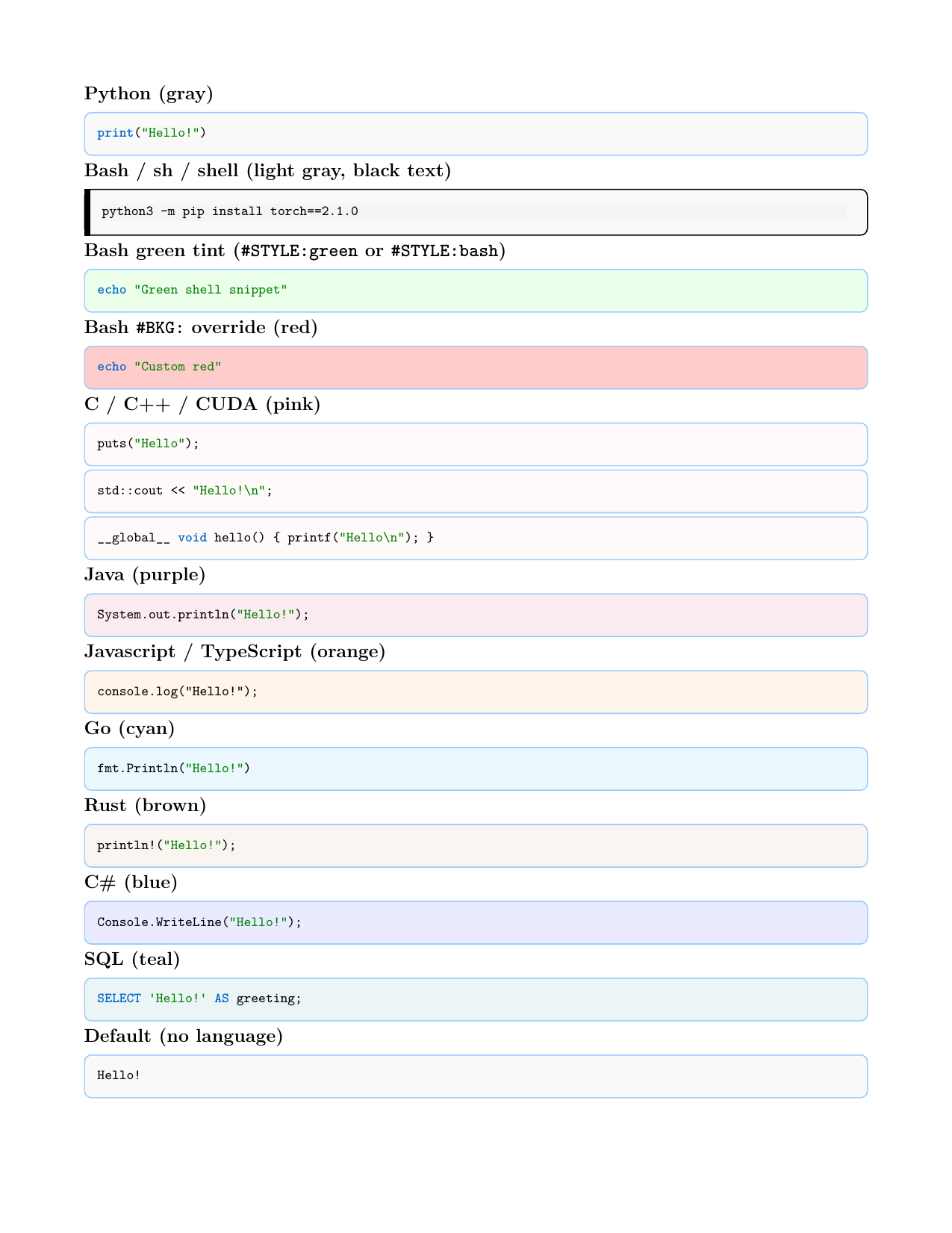
Code block styles in PDF: Python, bash, C++, Java, overrides, and terminal

Default by language¶

Language fence	PDF style
`python`	Gray box, blue border (default)
`bash`, `sh`, `shell`	Terminal style (light gray box, black text, black border, left accent bar)
`c`, `cpp`, `c++`, `cuda`	Light pink tint (`pink!8`) — shared C-family style
`java`	Light purple tint (`purple!8`)
`javascript`, `js`, `typescript`, `ts`	Light orange tint (`orange!8`)
`go`	Light cyan tint (`cyan!8`)
`rust`	Light brown tint (`brown!8`)
`csharp`, `cs`	Light blue tint (`blue!8`)
`sql`	Light teal tint (`teal!8`)
(none)	Gray box, blue border (same as `python` default)

```python
def greet(name: str) -> None:
    print(f"Hello, {name}!")
```

```bash
conda activate usao
python -m cibuildwheel --output-dir dist
```

```c
#include <stdio.h>
int main(void) { puts("hi"); return 0; }
```

```cpp
#include <iostream>
int main() { std::cout << "hi\n"; }
```

```cuda
__global__ void hello() { printf("hi\n"); }
```

```java
public class Main {
    public static void main(String[] args) { }
}
```

```typescript
const greet = (name: string): void => console.log(name);
```

```go
package main
func main() { fmt.Println("hi") }
```

```rust
fn main() { println!("hi"); }
```

```csharp
Console.WriteLine("hi");
```

```sql
SELECT 'hi' AS greeting;
```

```
plain text or unknown language
```

Custom background (`#BKG:`)¶

Add #BKG: as the first line inside the fence. Colors use LaTeX/xcolor names (e.g. red!20, yellow!20, gray!10).

```bash
#BKG:red!20
#STYLE:bash
echo "Custom red background"
```

bash / sh / shell default to terminal style (light gray background, black text, black border, left accent bar). A custom #BKG: tint keeps terminal highlighting. Add #STYLE:bash or #STYLE:green on the next line for the green-tinted shell look with bash syntax highlighting.

Combine with line-number markers: #BKG:red!20;#LINENUM or #BKG:red!20;#LINENUM;#LINEBAR.

Terminal style (default for `bash`, `sh`, `shell`)¶

bash, sh, and shell fences use the terminal look by default — light gray background with black text, a black border, and a left accent bar. Text is uniform (no bash syntax lexer, so digits, hyphens, and flags stay readable on the light background).

Bash line wrapping¶

Long lines are auto-wrapped only at spaces with a trailing \ on continued lines when bash_wrap_columns is set in merged peanut.config (default 76 in peanut.config.default; set null or 0 to disable). Continuation lines are indented two spaces.

Case	Behavior
Single long command	Wrapped at spaces with `\`
Multi-line script (`#SBATCH`, `export`, …)	Each long non-`#` line wrapped independently; `#` comment lines unchanged; separate commands are not joined with `\`
Lines already continued with `\`	Treated as one logical command, then wrapped if still too long

Add #NOWRAP as the first line inside the fence to skip auto-wrap for that block.

```bash
torchrun --nnodes=2 --nproc_per_node=8 --node_rank=0 \
  --master_addr=<master_ip> --master_port=29500 train.py
```

```bash
#!/bin/bash
#SBATCH --nodes=4
srun torchrun --nnodes=$SLURM_NNODES --nproc_per_node=8 \
  --node_rank=$SLURM_NODEID --master_addr=$MASTER_ADDR train.py
```

```bash
#NOWRAP
torchrun --nnodes=2 --very-long-flags ...
```

Useful for shell sessions, cluster commands, SLURM scripts, or log snippets.

```bash
conda activate usao
python -m cibuildwheel --output-dir dist
```

Green bash tint (`#STYLE:green` or `#STYLE:bash`)¶

For the older light-green shell box, add a style marker as the first line inside the fence:

```bash
#STYLE:green
echo "Light green background"
```

Terminal style (`#STYLE:terminal`)¶

Explicit terminal marker (same as the default for bash / sh / shell):

```bash
#STYLE:terminal
# List InfiniBand devices
ibdev2netdev
ib_write_bw <other_node_ip>
```

Works with any fenced language, not only bash.

No border radius (`#STYLE:no-border-radius`)¶

Square corners on the code box (overrides the default rounded border). Language background tints still apply.

```python
#STYLE:no-border-radius
print("Hello!")
```

No border line (`#STYLE:no-border-line`)¶

Removes the colored border line around the code box. Language background tints still apply.

```python
#STYLE:no-border-line
print("Hello!")
```

Preview fixture¶

To regenerate the preview PDF locally (from the peanutbook source repo):

./scripts/test_codeblock_styles.sh

Output: test_codeblock_styles.pdf and tests/output/codeblock_styles-*.png.

Mermaid diagrams¶

Fenced blocks tagged mermaid are rendered to PNG figures when you build — not shown as code listings. The same diagram source is used for PDF, DOCX, EPUB, and HTML output formats.

Basic usage¶

Mermaid flowchart example in PDF

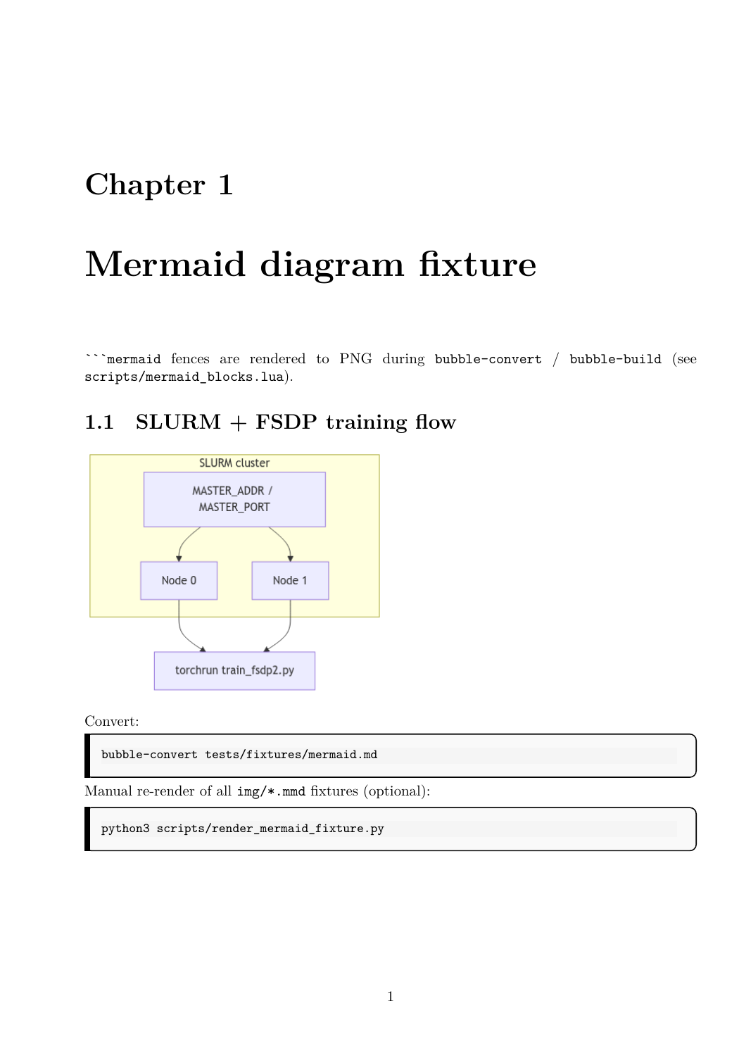
```mermaid
flowchart LR
  A[Master] --> B[Worker]
```

```{.mermaid width=50%}
flowchart TB
  subgraph cluster["SLURM cluster"]
    M["MASTER_ADDR / MASTER_PORT"]
    W1["Node 0"]
    W2["Node 1"]
    M --> W1
    M --> W2
  end
  W1 --> T["torchrun train_fsdp2.py"]
  W2 --> T
```

Language tag: mermaid (or class .{.mermaid}).
Optional attributes on the fence: width=50%, width=5cm, align=center (same as image attributes).
Default width when omitted: 90% of line width.

Building¶

Use the same Markdown in your chapter files as for PDF:

bubble-convert 1                    # chapter PDF
bubble-convert chapter.md --format docx
bubble-build                        # full book PDF
bubble-build --format epub
bubble-build --format docx
bubble-render-html                  # static HTML site
bubble-build --format html

Rendered PNGs are cached under each chapter’s img/.mermaid/ (content-hash filenames). Unchanged diagrams are not re-rendered.

Requirements: mermaid-cli (mmdc on PATH) or Node.js with npx. See System requirements — Mermaid. No extra peanut.config keys.

If Mermaid is not installed, PDF/DOCX/EPUB may leave the fence as a code block; HTML build logs an error and keeps the fence text.

Standalone diagram files (optional)¶

You can maintain diagrams as img/*.mmd and reference the exported PNG with ordinary Markdown images (![](img/diagram.png)), instead of or in addition to fenced blocks.

SVG (manual)¶

For vector figures in PDF, export SVG with mmdc and use ![](img/diagram.svg) where your template supports it. If PDF text misaligns, run bubble-convert-svg-text on the SVG.

Code Line Annotations¶

By default, code blocks do not display line numbers. Line numbers are automatically enabled when: 1. The code block is followed by a CODE_EXPLAIN_START block, or 2. You explicitly add LINENUM marker in the code block

Basic Usage (No Line Numbers):

```python
print("Hello")
print("World")
```

With Explanations (Line Numbers Auto-Enabled):

```python
print("Hello")
print("World")
```

CODE_EXPLAIN_START:

- 1: First line prints Hello
- 2: Second line prints World

CODE_EXPLAIN_END

Explicitly Enable Line Numbers:

Locally (per code block): Add #LINENUM at the beginning of the code block:

```python
#LINENUM
print("Hello")
print("World")
```

Globally (for all code blocks): Add "code_line_numbers": true to peanut.config:

"code_line_numbers": true

When enabled globally, line numbers are added to all Python code blocks by default. You can still disable line numbers locally on specific blocks by writing #NOLINENUM at the start of the block.

You can also combine it with background color specification:

```python
#BKG:yellow!20;#LINENUM
print("Hello")
print("World")
```

Disable Line Numbers (Override):

If you want to disable line numbers even when CODE_EXPLAIN_START is present, add NOLINENUM:

```python
#NOLINENUM
print("Hello")
print("World")
```

CODE_EXPLAIN_START:

- 1: First line prints Hello
- 2: Second line prints World

CODE_EXPLAIN_END

Line Number Style (Bar Style):

By default, line numbers and explanations are displayed as circled numbers (①, ②, ③, etc.). To use a box style (e.g., 13 or 1 in a box), you can configure it:

Locally (per code block): Add #LINEBAR in the first line comment:

```python
#LINEBAR
print("Hello")
print("World")
```

Globally (for the entire book): Set the "code_annotation_style" key in peanut.config to "bar" (or "box"):

"code_annotation_style": "bar"

Supported global values in peanut.config: - "circle": Force circled annotations. - "bar" or "box": Force boxed/bar annotations. - null (default): Determine style dynamically per-code-block (uses circle style unless #LINEBAR is specified in the code block).

Equation Numbering¶

Add numbered equations with labels and cross-references in your markdown.

Adding Equation Labels¶

To add a numbered equation, use $$...$$ for display math and include \label{eq:name} inside the formula:

$$
A = U \Sigma V^\top \label{eq:svd-full}
$$

Alternative Format: WFHLABEL

You can also use the \\WFHLABEL:eq:name format at the end of the equation line:

$$
A = U \Sigma V^\top \\WFHLABEL:eq:svd-full
$$

Both formats (\label{eq:name} and \\WFHLABEL:eq:name) are equivalent and will produce the same numbered equation. The WFHLABEL format is placed at the end of the equation line, while \label can be placed anywhere within the formula block.

CRITICAL REQUIREMENT: The formula block must have empty lines before and after it. This is essential for the Lua filter to correctly detect and process the equation:

Some text before the formula.

$$
A = U \Sigma V^\top \label{eq:svd-full}
$$

Some text after the formula.

Common Mistakes:

❌ No empty line before: Formula won't be detected

The formula is:
$$
A = U \Sigma V^\top \label{eq:svd-full}

❌ No empty line after: Formula won't be detected

$$
A = U \Sigma V^\top \label{eq:svd-full}
$$
This text follows immediately.

⚠️ Comma before label (style): This is usually valid LaTeX, but not recommended in Peanutbook style. Prefer no punctuation before \label for cleaner reading.
```
$$
A = U_k \Sigma_k V_k^\top, \label{eq:svd-thin}
$$
```

✅ Preferred format (empty lines required, no comma before label):

Some text before.

$$
A = U \Sigma V^\top \label{eq:svd-full}
$$

Some text after.

Referencing Equations¶

Reference numbered equations using @eq:name:

According to equation @eq:svd-full, we can decompose any matrix.

Or use LaTeX format:

According to equation \eqref{eq:svd-full}, we can decompose any matrix.

Both formats will be converted to proper LaTeX references with italic numbers.

Multi-line Equations¶

For multi-line equations with \begin{aligned} or \begin{align}, place the label at the end:

Using \label format:

$$
\begin{aligned}
V_\pi(s) &= \mathbb{E}_\pi[R_{t+1} + \gamma V_\pi(S_{t+1}) | S_t = s] \\
&= \sum_{a \in \mathcal{A}} \pi(a | s) \left[R(s, a) + \gamma \sum_{s' \in \mathcal{S}} P(s' | s, a) V_\pi(s')\right].
\end{aligned} \label{eq:bellman-state}
$$

Using WFHLABEL format:

$$
\begin{aligned}
V_\pi(s) &= \mathbb{E}_\pi[R_{t+1} + \gamma V_\pi(S_{t+1}) | S_t = s] \\
&= \sum_{a \in \mathcal{A}} \pi(a | s) \left[R(s, a) + \gamma \sum_{s' \in \mathcal{S}} P(s' | s, a) V_\pi(s')\right].
\end{aligned} \\WFHLABEL:eq:bellman-state
$$

Complete Example¶

### Singular Value Decomposition

Every matrix can be decomposed as:

$$
A = U \Sigma V^\top \label{eq:svd-full}
$$

where $U$ and $V$ are orthonormal matrices.

### Thin SVD

For economy-size decomposition:

$$
A = U_k \Sigma_k V_k^\top \label{eq:svd-thin}
$$

The relationship between @eq:svd-full and @eq:svd-thin is that the thin form uses only the first $k$ singular values.

NOTE: If the equation is not labeled and it use $$, there must be no empty line before the opening $$ and after the closing $$.

Important Notes¶

Label names must start with eq: (e.g., eq:svd-full, eq:norm)
Label names can only contain letters, numbers, underscores, and hyphens
Empty lines are mandatory before and after $$...$$ blocks - this is the only requirement
Style recommendation: no comma before label - a comma before \label{eq:name} or \\WFHLABEL:eq:name is usually valid, but Peanutbook recommends omitting it for cleaner formula typography
Two label formats are supported:
\label{eq:name} - can be placed anywhere in the formula
\\WFHLABEL:eq:name - placed at the end of the equation line
Indentation doesn't matter - as long as there are empty lines, formulas can be indented or not
Equation numbers are automatic - they increment sequentially within each chapter
References display as italic numbers in the PDF (e.g., "8.5" instead of "equation 8.5")

Technical Details¶

This feature is implemented via the equation_numbering.lua filter, which: - Detects display math blocks ($$...$$) containing \label{eq:...} - Converts them to LaTeX equation environments - Processes @eq:name references in text, converting them to \eqref{eq:name}

The filter is automatically applied when using bubble-convert or bubble-build.

Formula Annotations¶

Add visual annotations to mathematical formulas with arrows pointing to specific parts of the formula and descriptive text.

Basic Syntax¶

Place a fenced code block with identifier FORMULA-ANNO immediately after a display math block ($$...$$):

$$
KL(q||p) = \sum_{x} q(x) \log \frac{q(x)}{p(x)}
$$
```FORMULA-ANNO
above❤️q(x)❤️Approximating distribution
below❤️\frac{q(x)}{p(x)}❤️Log ratio of approximate to actual

### Annotation Format

Each annotation line follows the format:

position❤️formula_part❤️description

Where:
- `position`: Either `above` or `below` to indicate annotation position
- `formula_part`: The exact LaTeX code fragment from the formula to annotate (must match exactly)
- `description`: The annotation text to display
- `❤️`: Unicode heart emoji used as delimiter

### Configuration Options

You can configure various aspects of the annotations using option lines in the `FORMULA-ANNO` block:

**Vertical Spacing:**
```markdown
```FORMULA-ANNO
vspace-above:1cm
vspace-below:0.2cm
above❤️q(x)❤️Approximating distribution

- `vspace-above`: Vertical space above the formula (default: `0.5cm`)
- `vspace-below`: Vertical space below the formula (default: `0.5cm`)

**Colors:**
```markdown
```FORMULA-ANNO
color-above:blue
color-below:red
above❤️q(x)❤️Approximating distribution
below❤️\frac{q(x)}{p(x)}❤️Log ratio of approximate to actual

- `color-above`: Color for above annotations (default: black)
- `color-below`: Color for below annotations (default: black)
- Supports standard LaTeX color names (e.g., `blue`, `red`, `green`) or custom colors

**Arrow Styles:**
```markdown
```FORMULA-ANNO
arrow-style-above:curve
arrow-style-below:straight
above❤️q(x)❤️Approximating distribution

- `arrow-style-above`: Arrow style for above annotations (default: `curve`)
- `arrow-style-below`: Arrow style for below annotations (default: `curve`)
- Supported styles:
  - `straight`: Straight arrow pointing up/down
  - `curve`: Curved arrow with smooth ~150 degree turn
  - `L`: L-shaped arrow (vertical then horizontal)

**Arrow Directions:**
```markdown
```FORMULA-ANNO
arrow-direction-above:left
arrow-direction-below:right
arrow-style-above:curve
above❤️q(x)❤️Approximating distribution

- `arrow-direction-above`: Direction for above annotations (default: `left` for curve, can be `left` or `right`)
- `arrow-direction-below`: Direction for below annotations (default: `right` for curve, can be `left` or `right`)
- Only applies to `curve` and `L` arrow styles
- `left`: Arrow points to the left side
- `right`: Arrow points to the right side

### Complete Examples

**Example 1: Basic annotations with colors and spacing**
```markdown
$$
KL(q||p) = \sum_{x} q(x) \log \frac{q(x)}{p(x)}
$$
```FORMULA-ANNO
vspace-above:1cm
vspace-below:0.2cm
color-above:blue
color-below:red
arrow-style-above:curve
arrow-style-below:straight
arrow-direction-above:left
arrow-direction-below:right
above❤️q(x)❤️Approximating distribution
below❤️\frac{q(x)}{p(x)}❤️Log ratio of approximate to actual

**Example 2: L-shaped arrows**
```markdown
$$
L = \lim_{n \to \infty} \frac{1}{n} \sum_{i=1}^{n} x_i
$$
```FORMULA-ANNO
arrow-style-above:L
arrow-style-below:L
arrow-direction-above:left
arrow-direction-below:right
above❤️\lim_{n \to \infty}❤️Limit as n approaches infinity
below❤️\sum_{i=1}^{n}❤️Summation

**Example 3: Multiple annotations with default settings**
```markdown
$$
P = \prod_{i=1}^{n} x_i
$$
```FORMULA-ANNO
arrow-style-above:curve
arrow-style-below:curve
arrow-direction-above:left
arrow-direction-below:right
above❤️\prod_{i=1}^{n}❤️Product over all items
below❤️x_i❤️Individual variable

### Important Notes

1. **Exact Matching**: The `formula_part` must match exactly the LaTeX code in the formula, including all backslashes and special characters.

2. **Formula Part Matching**: The system uses exact string matching to find the formula part. Complex LaTeX commands like `\lim_{n \to \infty}` must be written exactly as they appear in the formula.

3. **Multiple Annotations**: You can have multiple `above` and `below` annotations in the same block.

4. **Visual Elements**:
   - A horizontal line (vertical bar) is drawn above/below the annotated formula part
   - A green dot (with 30% opacity) marks the center of the vertical bar
   - Arrows connect from the dot to the annotation text

5. **Arrow Behavior**:
   - **Straight arrows**: Point directly up/down from the formula
   - **Curved arrows**: Smooth ~150 degree turn, compact bend, never exceed annotation text height
   - **L-shaped arrows**: Vertical segment (0.3 units) then horizontal segment (2.0 units) to text
   - Left direction curves never extend beyond the vertical bar center in the x-axis direction

6. **Font**: Annotation text uses sans-serif, bold, small font size.

7. **Line Width**: Curve arrows use 0.5pt line width.

### Technical Details

- The annotation block must immediately follow the display math block
- The `FORMULA-ANNO` identifier is case-sensitive
- Configuration options are parsed line by line
- Empty lines in the annotation block are ignored
- The system uses TikZ with `tikzmarknode` to mark formula parts and draw annotations

## Table Width Control

Control table widths in your PDF output using fenced divs with width attributes.

### Syntax

Wrap your table in a fenced div with a `width` attribute:

````markdown
::: {width=80%}

| Column 1 | Column 2 | Column 3 |
|----------|----------|----------|
| Data 1   | Data 2   | Data 3   |
| Data 4   | Data 5   | Data 6   |

:::
````

### Width Formats

You can specify width in several formats:

- **Percentage**: `width=80%` (80% of text width)
- **Decimal**: `width=0.8` (equivalent to 80%)
- **LaTeX units**: `width=0.8\textwidth` (also equivalent to 80%)

**Examples:**

````markdown
::: {width=70%}

| Narrow Table | Content |
|--------------|---------|
| Row 1        | Data    |

:::

::: {width=0.9}

| Wide Table | Column 2 | Column 3 |
|------------|----------|----------|
| Data       | More     | Content  |

:::
````

### How It Works

1. The `table_width_div.lua` filter detects fenced divs with `width` attributes containing tables
2. It inserts a LaTeX comment (`% TABLE_WIDTH: 80%`) before the table
3. The `fix_table_width.py` script processes the LaTeX file and:
   - Converts table column specifications to `p{...}` format with proportional widths
   - Wraps the table in a `minipage` environment to constrain the overall width
   - Centers the table using a `center` environment

### Default Behavior

- **Without width attribute**: Tables default to 85% of text width with equal column widths
- **With width attribute**: Tables use the specified width, divided equally among columns

### Important Notes

1. **Fenced div syntax**: Use `:::` to create fenced divs (not code fences)
2. **Width attribute**: Must be specified as `width=X` where X is a percentage, decimal, or LaTeX unit
3. **Table must be inside div**: The table must be directly inside the fenced div
4. **Column widths**: Width is divided equally among all columns automatically
5. **Centering**: Tables with width attributes are automatically centered

### Complete Example

````markdown
Here is a narrow table:

::: {width=60%}

| Algorithm | Complexity | Space |
|-----------|------------|-------|
| Quick Sort | $O(n \log n)$ | $O(\log n)$ |
| Merge Sort | $O(n \log n)$ | $O(n)$ |
| Heap Sort  | $O(n \log n)$ | $O(1)$ |

:::

And here is a wider table:

::: {width=90%}

| Method | Advantages | Disadvantages |
|--------|------------|---------------|
| Method A | Fast | Memory intensive |
| Method B | Memory efficient | Slower |

:::
````

### Technical Details

- Implemented via `table_width_div.lua` (Pandoc filter) and `fix_table_width.py` (post-processing script)
- Automatically applied when using `bubble-convert` or `bubble-build`
- Works with Pandoc's `longtable` environment for multi-page tables

## Table References

Add numbered tables with captions and labels, and cross-reference them in your markdown.

### Adding Table Captions and Labels

To add a numbered table with a caption and label, use Pandoc's table syntax with a caption and identifier:

**Method 1: Table with Caption and Label**

````markdown
::: {width=80%}

| Column 1 | Column 2 | Column 3 |
|----------|----------|----------|
| Data 1   | Data 2   | Data 3   |
| Data 4   | Data 5   | Data 6   |

Table: Comparison of different methods {#tbl:comparison}

:::
````

**Method 2: Table Caption Only (No Label)**

````markdown
::: {width=80%}

| Algorithm | Complexity | Space |
|-----------|------------|-------|
| Quick Sort | $O(n \log n)$ | $O(\log n)$ |
| Merge Sort | $O(n \log n)$ | $O(n)$ |

Table: Time and space complexity comparison

:::
````

**Important Notes:**
- The caption line must start with `Table:` followed by the caption text
- To add a label, use `{#tbl:name}` after the caption text
- Label names must start with `tbl:` prefix (e.g., `tbl:comparison`, `tbl:complexity`)
- Label names can only contain letters, numbers, underscores, and hyphens
- The caption line should be placed immediately after the table (before the closing `:::` if using fenced div)

### Referencing Tables

Reference numbered tables using `@tbl:name`:

```markdown
As shown in Table @tbl:comparison, the methods differ significantly.

Or use LaTeX format:

As shown in Table~\ref{tbl:comparison}, the methods differ significantly.

Both formats will be converted to proper LaTeX references with "Table" prefix (e.g., "Table 1.2").

Complete Example¶

### Algorithm Complexity

The following table compares different sorting algorithms:

::: {width=70%}

| Algorithm | Time Complexity | Space Complexity |
|-----------|----------------|------------------|
| Quick Sort | $O(n \log n)$ | $O(\log n)$ |
| Merge Sort | $O(n \log n)$ | $O(n)$ |
| Heap Sort  | $O(n \log n)$ | $O(1)$ |
| Bubble Sort| $O(n^2)$ | $O(1)$ |

Table: Comparison of sorting algorithms {#tbl:sorting-algorithms}

:::

As shown in Table @tbl:sorting-algorithms, most efficient algorithms have $O(n \log n)$ time complexity.

Important Notes¶

Label names must start with tbl: (e.g., tbl:comparison, tbl:complexity)
Label names can only contain letters, numbers, underscores, and hyphens
Caption format: Use Table: Your caption text {#tbl:name} after the table
Table numbering is automatic - tables are numbered sequentially within each chapter
References display with "Table" prefix in the PDF (e.g., "Table 1.2" instead of just "1.2")
Works with table width control - you can combine width attributes with captions and labels

Technical Details¶

This feature uses: - Pandoc's native table caption support: Tables with captions are converted to LaTeX longtable with \caption{} - Pandoc's identifier system: Labels added via {#tbl:name} are converted to LaTeX \label{tbl:name} - figure_references.lua filter: Processes @tbl:name references in text, converting them to Table~\ref{tbl:name}

The filters are automatically applied when using bubble-convert or bubble-build.

Code Snippet References¶

Add labels to code blocks and cross-reference them in your markdown, similar to equations and tables.

Adding Code Block Labels¶

To add a label to a code block, use Pandoc's identifier syntax with {#code:name}:

```python {#code:example-print}
print(123)
```

Important Notes: - Label names must start with code: prefix (e.g., code:example-print, code:main-function) - Label names can only contain letters, numbers, underscores, and hyphens - The identifier {#code:name} is placed after the language specification - Works with any programming language (Python, JavaScript, Bash, etc.)

Referencing Code Snippets¶

Reference labeled code blocks using @code:name:

As shown in @code:example-print, we can print numbers.

Or use LaTeX format:

As shown in Code~\ref{code:example-print}, we can print numbers.

Important: When using @code:name, do not include "Code" in your text - the filter automatically adds the "Code" prefix. If you write "Code @code:name", it will result in "Code Code 1" in the output.

Both formats will be converted to proper LaTeX references with "Code" prefix (e.g., "Code 1.2").

Complete Example¶

### Function Definition

Here is a simple function:

```python {#code:hello-function}
def hello(name):
    print(f"Hello, {name}!")
```

### Function Usage

As shown in @code:hello-function, the function takes a name parameter and prints a greeting.

You can also reference it using LaTeX format: Code~\ref{code:hello-function}.

Important Notes¶

Label names must start with code: (e.g., code:hello-function, code:main)
Label names can only contain letters, numbers, underscores, and hyphens
Code numbering is automatic - code blocks are numbered sequentially within each chapter
References display with "Code" prefix in the PDF (e.g., "Code 1.2" instead of just "1.2")
Works with all code block features - labels work with line numbers, background colors, and other code block features

Technical Details¶

This feature uses: - code_labels.lua filter: Processes code blocks with identifiers and stores label information - code_line_numbers.lua filter: Adds LaTeX \label{} commands to code blocks when rendering - figure_references.lua filter: Processes @code:name references in text, converting them to Code~\ref{code:name}

The filters are automatically applied when using bubble-convert or bubble-build.

Algorithm Formatting¶

Format algorithms professionally using fenced code blocks with the algorithm class. Algorithms are automatically converted to LaTeX algorithm environments with proper formatting using the algorithmicx package.

Method 1: Fenced Code Block (Recommended)¶

Use a fenced code block with the algorithm class:

```{.algorithm caption="Gram–Schmidt Algorithm" label="alg:gram-schmidt"}
\Require A set of linearly independent vectors $\{\mathbf{v}_0, \ldots, \mathbf{v}_{r-1}\}$
\Ensure An orthonormal basis $\{\mathbf{e}_0, \ldots, \mathbf{e}_{r-1}\}$
\State $\mathbf{e}_0 \gets \frac{\mathbf{v}_0}{\|\mathbf{v}_0\|_2}$
\For{$i = 1, \ldots, r-1$}
    \State $\mathbf{R}_i \gets \mathbf{v}_i - \sum_{j=0}^{i-1} \langle \mathbf{v}_i, \mathbf{e}_j \rangle \mathbf{e}_j$
    \State $\mathbf{e}_i \gets \frac{\mathbf{R}_i}{\|\mathbf{R}_i\|_2}$
\EndFor
```

Method 2: Fenced Div (For Complex Layouts)¶

Use a fenced div with the algorithm class:

::: {.algorithm caption="Gram–Schmidt Algorithm" label="alg:gram-schmidt"}
```latex
\Require A set of linearly independent vectors $\{\mathbf{v}_0, \ldots, \mathbf{v}_{r-1}\}$
\Ensure An orthonormal basis $\{\mathbf{e}_0, \ldots, \mathbf{e}_{r-1}\}$
\State $\mathbf{e}_0 \gets \frac{\mathbf{v}_0}{\|\mathbf{v}_0\|_2}$
\For{$i = 1, \ldots, r-1$}
    \State $\mathbf{R}_i \gets \mathbf{v}_i - \sum_{j=0}^{i-1} \langle \mathbf{v}_i, \mathbf{e}_j \rangle \mathbf{e}_j$
    \State $\mathbf{e}_i \gets \frac{\mathbf{R}_i}{\|\mathbf{R}_i\|_2}$
\EndFor
```
:::

Attributes¶

Both methods support the following attributes:

caption: The algorithm caption (e.g., "Gram–Schmidt Algorithm")
label: The LaTeX label for cross-referencing (e.g., "alg:gram-schmidt")

Algorithmicx Commands¶

The following commands are available (using algpseudocode style):

Input/Output: - \Require{...} - Input requirement (displays as "Input:") - \Ensure{...} - Output guarantee (displays as "Output:")

Control Structures: - \State - Regular statement - \If{condition} ... \EndIf - If statement - \If{condition} ... \Else ... \EndIf - If-else statement - \For{condition} ... \EndFor - For loop - \While{condition} ... \EndWhile - While loop - \Repeat ... \Until{condition} - Repeat-until loop

Comments: - \Comment{...} - Inline comment (displays with ▷ symbol)

Examples¶

Simple algorithm:

```{.algorithm caption="Vector Normalization" label="alg:normalize"}
\Require Vector $\mathbf{v} \in \mathbb{R}^d$
\Ensure Unit vector $\hat{\mathbf{v}}$
\State $\hat{\mathbf{v}} \gets \frac{\mathbf{v}}{\|\mathbf{v}\|_2}$
\State \Return $\hat{\mathbf{v}}$
```

Algorithm with loops:

```{.algorithm caption="Gram–Schmidt Process" label="alg:gram-schmidt"}
\Require Linearly independent vectors $\{\mathbf{v}_0, \ldots, \mathbf{v}_{r-1}\}$
\Ensure Orthonormal basis $\{\mathbf{e}_0, \ldots, \mathbf{e}_{r-1}\}$
\State $\mathbf{e}_0 \gets \frac{\mathbf{v}_0}{\|\mathbf{v}_0\|_2}$ \Comment{Normalize first vector}
\For{$i = 1, \ldots, r-1$}
    \State $\mathbf{R}_i \gets \mathbf{v}_i$
    \For{$j = 0, \ldots, i-1$}
        \State $\mathbf{R}_i \gets \mathbf{R}_i - \langle \mathbf{v}_i, \mathbf{e}_j \rangle \mathbf{e}_j$ \Comment{Remove projection}
    \EndFor
    \State $\mathbf{e}_i \gets \frac{\mathbf{R}_i}{\|\mathbf{R}_i\|_2}$ \Comment{Normalize residual}
\EndFor
```

Algorithm with conditionals:

```{.algorithm caption="Safe Division" label="alg:safe-divide"}
\Require $a, b \in \mathbb{R}$
\Ensure $c = a / b$ if $b \neq 0$, error otherwise
\If{$b = 0$}
    \State \Return error \Comment{Division by zero}
\Else
    \State $c \gets a / b$
    \State \Return $c$
\EndIf
```

Cross-Referencing¶

You can reference algorithms using standard LaTeX syntax:

As shown in Algorithm~\ref{alg:gram-schmidt}, the process...

Or using Pandoc citation syntax (if supported):

As shown in @alg:gram-schmidt, the process...

Best Practices¶

Always include a caption: Makes algorithms easier to reference
Use descriptive labels: Use format alg:algorithm-name for consistency
Keep algorithms focused: Each algorithm should solve one specific problem
Use comments sparingly: Only add comments when they add clarity
Format math properly: Use LaTeX math mode for all mathematical expressions
Indent nested structures: Use consistent indentation (typically 4 spaces)

Technical Details¶

The filter algorithm_blocks.lua processes algorithm blocks
Algorithms are converted to LaTeX algorithm environment
The algorithmicx package with algpseudocode style is used
Algorithms are automatically numbered and can be cross-referenced
The filter is automatically applied when using bubble-convert or bubble-build

For more detailed information, see docs/algorithm_usage.md.

Definition, Theorem, Example, and Property References¶

Add cross-references to definitions, theorems, examples, and properties using LaTeX labels and references.

Adding Labels to Headings¶

To add a label to a definition, theorem, example, or property, use Pandoc attribute syntax with {#prefix:name}:

### Definition: Determinant {#def:determinant}

### Theorem: Spectral Radius {#thm:spectral-radius}

#### Example: RoPE in Transformers {#ex:rope-transformers}

### Property: Idempotency {#prop:idempotency}

Label naming conventions: - Definitions: use def: prefix (e.g., def:determinant) - Theorems: use thm: prefix (e.g., thm:spectral-radius) - Examples: use ex: prefix (e.g., ex:rope-transformers) - Properties: use prop: prefix (e.g., prop:idempotency) - Label names can only contain letters, numbers, underscores, and hyphens

Referencing¶

Reference these elements using the LaTeX \ref command:

The **determinant** was formally defined in Chapter 5 (see Definition~\ref{def:determinant}).

According to Theorem~\ref{thm:spectral-radius}, the spectral radius equals the maximum absolute eigenvalue.

For a detailed implementation, see Example~\ref{ex:rope-transformers}.

The projection matrix satisfies the idempotency property (see Property~\ref{prop:idempotency}).

Reference format: - Use Definition~\ref{def:name} for definitions - Use Theorem~\ref{thm:name} for theorems - Use Example~\ref{ex:name} for examples - Use Property~\ref{prop:name} for properties - The ~ (tilde) creates a non-breaking space between the label and the number - References will display as section or subsection numbers (e.g., "Definition 5.1", "Property 2.4.1")

Cross-Chapter References¶

You can reference elements from other chapters:

The determinant was formally defined in Chapter 5 (see Definition~\ref{def:determinant}).
Here we explore its geometric interpretation.

LaTeX will automatically handle cross-chapter references and display the correct chapter and section numbers.

Important Notes¶

Label names should use prefixes: def: for definitions, thm: for theorems, ex: for examples
Labels are added to headings: Use {#prefix:name} after the heading text
Use ~ for non-breaking space: Definition~\ref{def:name} prevents line breaks
Cross-chapter references work automatically: LaTeX handles chapter numbers
References display as section/subsection numbers: The reference will show the number where the element appears

Technical Details¶

This feature uses Pandoc's native label and reference system: - Labels are added using Pandoc attribute syntax {#def:name} or {#thm:name} - Pandoc converts these to LaTeX \label{def:name} or \label{thm:name} - References using \ref{def:name} or \ref{thm:name} are processed by LaTeX - LaTeX automatically resolves cross-references and displays section numbers

No special Lua filter is needed—this works with Pandoc's built-in cross-reference support.

Footnotes¶

Add footnotes using standard Pandoc syntax:

This is some text with a footnote[^1].
More text with another footnote[^2].

[^1]: This is the first footnote.
[^2]: This is the second footnote.

Footnotes will automatically appear at the bottom of each page in the PDF.

Lists After Colons¶

CRITICAL REQUIREMENT: When introducing a list with a colon (:) followed by a newline, you must have an empty line between the colon and the list. This ensures proper Markdown parsing and consistent formatting in the PDF output.

Common Patterns: - where: followed by a list - For example: followed by a list - Note: followed by a list - Any text ending with : that introduces a list

BAD:

where:
- a
- b

Good:

where:

- a
- b

Common Mistakes:

❌ No empty line after colon: List may not be properly formatted
```
where:
- item 1
- item 2
```
✅ Empty line after colon: Correct formatting
```
where:

- item 1
- item 2
```

Keyword Indexing¶

Create a professional keyword index at the end of your book using bracketed span syntax.

Syntax¶

Wrap any word or phrase in brackets followed by the {.idx} or {.index} class:

Linear algebra is the study of [vector spaces]{.idx}.
The [Singular Value Decomposition]{.index} is a key tool in ML.

Features¶

Normalization: All index entries are automatically normalized to lowercase in the index to ensure terms like "Vector" and "vector" are merged into a single entry with multiple page numbers.
Placement: The index is automatically generated and placed at the very end of the book (before the back cover).
Case Sensitivity: While the index listing is lowercase for better grouping, the text in your chapters remains exactly as you typed it.

Semantic Chapter References¶

Refer to chapters by their topic instead of hardcoded numbers to ensure your text stays accurate when chapters are moved or reordered.

Syntax¶

Use the LaTeX \ref command with the chap: prefix followed by the folder's slug (the descriptive part of the directory name after chapterN-).

As discussed in Chapter \ref{chap:matrix}, matrices represent linear maps.
See Chapter \ref{chap:svd} for applications in data compression.

Slug Examples¶

The slug is derived from the directory name: - chapter1-vector-space-inner-product $\to$ chap:vector-space-inner-product - chapter2-matrix $\to$ chap:matrix - chapter8-svd $\to$ chap:svd

Features¶

Automatic Labeling: Every chapter is automatically assigned a label based on its folder name.
Numerical Reference: Numbers in the final PDF are generated by LaTeX at build time, so they are always correct regardless of the folder's index.
Fallback: You can also use numerical labels like \ref{chap:1}, but slug-based labels are recommended for better readability and maintenance.

Conditional Markdown Includes¶

Conditionally include external markdown files based on configuration settings. This enables you to maintain multiple document variants (e.g., student version vs. instructor version, basic vs. advanced) from a single source.

Syntax¶

Use HTML comments in your markdown files to specify conditional includes:

<!-- include: path/to/file.md if condition_name -->

Syntax Details: - Format:  - File path: Relative to the current markdown file's directory - Condition: A boolean flag name defined in the config file - Multiple conditions: Use and, or, not operators:

<!-- include: advanced.md if advanced_mode and show_details -->
<!-- include: appendix.md if include_appendix or debug_mode -->
<!-- include: notes.md if not student_version -->

Examples¶

Basic include:

# Chapter 1: Introduction

This is the main content.

<!-- include: exercises.md if include_exercises -->

More content here.

Include with multiple conditions:

<!-- include: solutions.md if instructor_mode and show_solutions -->

Include with negation:

<!-- include: advanced_topics.md if not basic_version -->

Configuration File¶

Create a JSON configuration file (default: peanut.config in the project root) to define conditions:

{
  "include_math": true,
  "include_numpy": false,
  "include_torch": false,
  "include_exercises": true,
  "include_solutions": false,
  "instructor_mode": false,
  "advanced_mode": true
}

Configuration File Location: 1. Default location: peanut.config in the project root 2. Custom location: Specify with --include-config or -c flag when using bubble-convert:

bubble-convert 1 --include-config custom.config

Configuration File Format: - Format: JSON (file extension is .config but content is JSON) - Values: Boolean (true/false) or string values - Condition evaluation: - true → condition is met - false → condition is not met

Usage Examples¶

Student vs. Instructor Versions:

student.config:

{
  "include_exercises": true,
  "include_solutions": false,
  "include_hints": true
}

instructor.config:

{
  "include_exercises": true,
  "include_solutions": true,
  "include_hints": false,
  "include_notes": true
}

chapter1.md:

# Chapter 1: Linear Algebra

Main content here.

<!-- include: exercises.md if include_exercises -->
<!-- include: solutions.md if include_solutions -->
<!-- include: hints.md if include_hints -->
<!-- include: instructor_notes.md if include_notes -->

Generate different PDFs:

bubble-convert 1 --include-config student.config
bubble-convert 1 --include-config instructor.config

Basic vs. Advanced Content:

basic.config:

{
  "basic_version": true,
  "include_advanced": false
}

advanced.config:

{
  "basic_version": false,
  "include_advanced": true
}

chapter2.md:

# Chapter 2: Matrix Decomposition

Basic content here.

<!-- include: advanced_topics.md if include_advanced -->

Nested Includes¶

Included files can themselves contain include directives:

main.md:

<!-- include: section1.md if include_section1 -->

section1.md:

# Section 1

<!-- include: subsection1.md if show_details -->

File Path Resolution¶

Include paths are relative to the markdown file's directory
Example: If chapter1/chapter1.md includes exercises.md, it looks for chapter1/exercises.md
Absolute paths are also supported

Error Handling¶

Missing config file: If no config file is found, all includes are skipped (no error). The bubble package provides a default peanut.config.default that will be used as a fallback.
Missing include file: Warning is shown, include directive is removed
Invalid condition: Warning is shown, include directive is removed
Circular includes: Detected and prevented (max depth: 10 levels)

Processing Order¶

Include processing happens first (before chapter title extraction)
Chapter title extraction runs on the processed file
Pandoc conversion uses the final processed markdown

Best Practices¶

Use descriptive condition names: include_exercises is better than ex1
Document your conditions: Add comments in config files explaining what each flag does
Test with different configs: Verify your document works with various condition combinations
Keep includes simple: Avoid deeply nested includes (max 3-4 levels recommended)
Use relative paths: Keep your project portable by using relative paths

Troubleshooting¶

Include not working: 1. Check that the config file exists and is valid JSON 2. Verify the condition name matches exactly (case-sensitive) 3. Check that the file path is correct (relative to markdown file) 4. Look for warnings in the script output

Circular include detected: - Check for files that include each other - Reduce nesting depth - Restructure your includes to avoid cycles

File not found: - Verify the path is relative to the markdown file's directory - Check file permissions - Ensure the file extension is .md

Technical Details¶

Implemented via process_includes.py script
Automatically applied when using bubble-convert or bubble-build
Supports recursive includes up to 10 levels deep
Preserves line numbers for better error messages

For more detailed information, see docs/conditional_includes.md.

Peanutbook syntax reference¶

Syntax for NOTE Sections: NOTES-NOTEE format¶

Syntax for IMPORTANT Sections: IMPORS-IMPORE format¶

Syntax for WARNING Sections: WARNS-WARNE format¶

Syntax for page-centered blocks: CENTERS-CENTERE format¶

Syntax for IMAGE Attributes¶

Syntax for Fancy Divider¶

Code Block Styles¶

Default by language¶

Custom background (#BKG:)¶

Terminal style (default for bash, sh, shell)¶

Bash line wrapping¶

Green bash tint (#STYLE:green or #STYLE:bash)¶

Terminal style (#STYLE:terminal)¶

No border radius (#STYLE:no-border-radius)¶

No border line (#STYLE:no-border-line)¶

Preview fixture¶

Mermaid diagrams¶

Basic usage¶

Building¶

Standalone diagram files (optional)¶

SVG (manual)¶

Code Line Annotations¶

Equation Numbering¶

Adding Equation Labels¶

Referencing Equations¶

Multi-line Equations¶

Complete Example¶

Important Notes¶

Technical Details¶

Formula Annotations¶

Basic Syntax¶

Complete Example¶

Important Notes¶

Technical Details¶

Code Snippet References¶

Adding Code Block Labels¶

Referencing Code Snippets¶

Complete Example¶

Important Notes¶

Technical Details¶

Algorithm Formatting¶

Method 1: Fenced Code Block (Recommended)¶

Method 2: Fenced Div (For Complex Layouts)¶

Attributes¶

Algorithmicx Commands¶

Examples¶

Cross-Referencing¶

Best Practices¶

Technical Details¶

Definition, Theorem, Example, and Property References¶

Adding Labels to Headings¶

Referencing¶

Cross-Chapter References¶

Important Notes¶

Technical Details¶

Footnotes¶

Lists After Colons¶

Keyword Indexing¶

Syntax¶

Features¶

Semantic Chapter References¶

Syntax¶

Slug Examples¶

Features¶

Conditional Markdown Includes¶

Syntax¶

Examples¶

Configuration File¶

Usage Examples¶

Nested Includes¶

File Path Resolution¶

Error Handling¶

Processing Order¶

Best Practices¶

Troubleshooting¶

Technical Details¶

Custom background (`#BKG:`)¶

Terminal style (default for `bash`, `sh`, `shell`)¶

Green bash tint (`#STYLE:green` or `#STYLE:bash`)¶

Terminal style (`#STYLE:terminal`)¶

No border radius (`#STYLE:no-border-radius`)¶

No border line (`#STYLE:no-border-line`)¶